WIPP Actuator Disk Detailed Results
WIPP Test Case
This test case was part of the Workshop for Integrated Propeller Prediction (WIPP) and results are documented in the paper entitled: "Comparison of Propeller-Wing Interaction Simulation using Different Levels of Fidelity", Z. Yang, A. Kirby and D. Mavriplis, AIAA paper 2022-1678, DOI: 10.2514/6.2022-1678, available at: https://scientific-sims.com/cfdlab/Dimitri_Mavriplis/HOME/assets/papers/6.2022-1678.pdf
The test case is described in detail in the paper and a detailed explanation of the input files and parameters is given in the documentation on Actuator Disk Test Cases. Here we focus on the results of the CFD simulations for this case and highlight the differences between the various actuator disk methods.
Three methods are used to run this case:
- Assumed Load Distribution (loadtype=2) (Case 1)
- Prescribed Load Distribution (loadtype=4) (Case 2)
- Blade-element Theory Loading (loadtype=3) (Case 3 and Case 4)
The test case corresponds to RUN 180 in the WIPP workshop and defined in AIAA paper 2022-1678. The conditions for this case are:
- Mach = 0.08
- Angle of Attack = 0.0 deg.
- Reynolds Number = 567,801/ft
- Thrust Coefficient CT = 0.4
The thrust coefficient definition for the workshop is different than that used by the actuator disk code.
- Workshop CT = Thrust / (1/2 rho U^2 Area) where rho is the freestream density, U is the freestream velocity and Area is given as 675.6 in^2. This reference area is the same as that used in the definition of the wing component lift and drag coefficients of the WIPP geoemtry, and is thus not a characteristic of the actuator disk or rotor geometry.
The CFD solution was first run in the absence of the actuator disk for 100, 100 and 3000 multigrid cycles on the progressively finer grids of the multigrid sequence to establish the baseline flow field. The actuator disk runs were then restarted with from this (unpowered) flow field and run for 5000 multigrid cycles.
The NSU3D input file for these runs is shown below:
1                      NSU3D INPUT FILE: WIPP TEST CASE with Actuator Disk
2  RESTARTF  RESTARTT  RNTCYC
3  1.0       1.0       00.
4  RESTART FILE
5  ./WRKr/restart.out
6  MMESH     NTHREAD
7  1.0       1.0              (1st order = -1)
8  NCYC      NPRNT     N MESH    MESHLEVEL   CFLMIN    RAMPCYC   TURBFREEZE   FVIS2  FSOLVER_TYPE
9  5000.     0.0        4.        1.0        1.0       0.0       0.           0.      0.0
10 CFL       CFLV      ITACC     INVBC     ITWALL    TWALL
11 1.0        1000.      0.0       0.0       0.0     0.0
12 VIS 1     VIS 2     H FACTOR  SMOOP     NCYCSM
13 0.0        10.        0.00    0.00      0.0
14 C1        C2        C3        C4        C5        C
15 0.5321    1.3711    2.7744
16 FIL1      FIL2      FIL3      FIL4      FIL5      FIL6
17 1.0       1.0       1.0
18 ----------------------------------------------------------------------
19 COARSE LEVEL AND MULTIGRID PARAMETERS
20 CFLC      CFLVC     SMOOPC    NSMOOC
21 1.0       1000.     0.0       0.0
22 VIS0      MGCYC     SMOOMG    NSMOOMG
23 4.0       2.        0.8       2.0
24 ----------------------------------------------------------------------
25 TURBULENCE EQUATION(S)
26 ITURB     IWALLF    WALLDIST
27 4.        0.0        1.0
28 CT1       CT2        CT3      CT4       CT5       CT6
29  1.0      1.0        1.0      0.0       0.0
30 CTC1      CTC2       CTC3     CTC4      CTC5      CTC6
31 1.0       1.0        1.0      0.0       0.0
32 VIST0  TSMOOMG   NTSMOOMG
33 2.0        0.8        2.0
34 ----------------------------------------------------------------------
35 MACH      Z-ANGLE   Y-ANGLE   RE       RE_LENGTH
36 0.08      0.        0.00      0.567801e6    12.
37 ----------------------------------------------------------------------
38 FORCE/MOMENT COEFFICIENT PARAMETERS
39 REF_AREA  REF_LENGTH XMOMENT  YMOMENT   ZMOMENT  ISPAN
40 675.6     11.6       2.99     6.35      0.28     2.0
41 ----------------------------------------------------------------------
42 OPTIONAL ACTUATOR DISK PARAMETERS
43 IDISK_TYPE IDISK_START IDISK_FREQ IDISK_TRIM IDISK_FM
44 1.0        0.0         1.0        0.0        0.0
45 ----------------------------------------------------------------------
46 MESH DATA FILE
47 ../../grids/PWIX_DSV2_AIL0_NP_F_R0p70_FUN3D.part.320
48 ----------------------------------------------------------------------
49 OPTIONAL PARAMETERS (MODIFY FROM DEFAULT VALUES SET IN set_lim_values.f)
50 PARAMETER NAME                           VALUE(real number with decimal)
51 ISAFE_MG                                  1.0
52 IN_SITU_POST_PROC                         1.0


..
The actuator disk parameters are set in the input.actdisk file, and are described in detail in the Actuator Disk Cases documentation section.
Figure 1 illustrates the flow solution for the blade-element loading case colored by Mach number on the z=0.0 cutting plane, where the wake induced by the actuator disk is visualized.
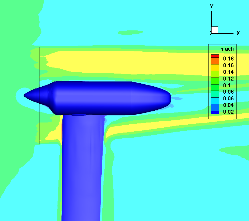
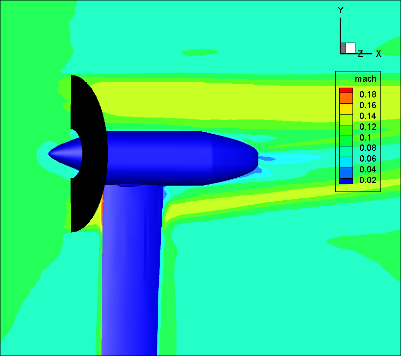
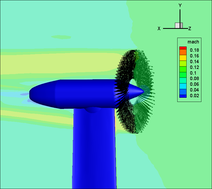
Figure 1: Illustration of actuator disk solution for WIPP case with blade-element loading.
Figure 2 depicts the convergence history for both the prescribed load case (Case 2) and the blade-element loading case (Case 3). Here the convergence history includes the initial unpowered solution history, which is identical for both cases, afterwhich small differences are seen between the two cases once the actuator disk is invoked. This figure shows that the convergence histories are similar for both actuator disk cases.
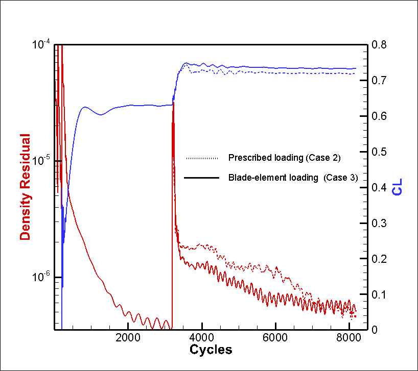
Figure 2: Convergence histories for prescribed loading and blade-element loading actuator disk cases.
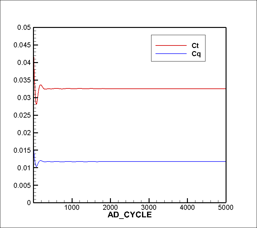
Figure 3: Convergence history of actuator disk thrust and torque coefficients for blade-element loading case.
Figure 3 depicts the convergence of the actuator disk thrust and torque coefficients, as defined in the actuator disk code, which is different than the CT defined by the workshop. These nondimensional coefficients are defined as:
- Thrust Coefficient: Ct = Thrust / (reference density x (Blade Tip Velocity)^2 x Disk Area) or Ct = Thrust / (reference density x Omega^2 x pi x Disk Radius^4)
- Moment Coefficient: Cq = Moment / (reference density x (Blade Tip Velocity)^2 x Disk Area x Disk Radius)
As can be seen from the figure, these computed disk coefficients converge quickly for the blade-element loading case. Note that for prescribed loading cases, the computed disk loading is constant and independent of the CFD flowfield solution.
Detailed Comparison
Results for the power-off (no disk) baseline case are discussed first. For this case, the values of lift and drag coefficients are given as:
- CL = 0.5926
- CD = 0.0293
Note that these values do not include the forces on the "standoff" component, illustrated in the figure below, as per the workshop guidelines. (The convergence plot in Figure 2 includes CL for all wetted surfaces). These values are obtained by subtracting the standoff component force contributions from the overall force coefficents reported in the force1.out file, as read from the comp.force.wind.out file (values on the last line of the "Standoff" component entries, at the last recorded solver iteration at the end of the file).
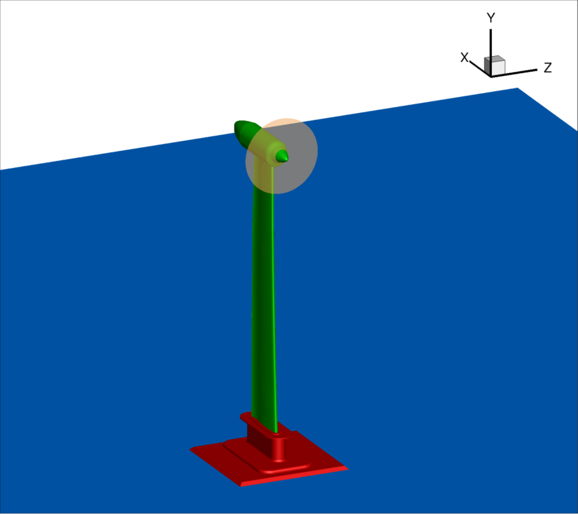
Figure 4: Illustration of standoff component (in red) to be excluded from force integration.
The comparison of power off (CT=0.0) predicted lift and drag coefficients with experimental data is given in Figure 5.
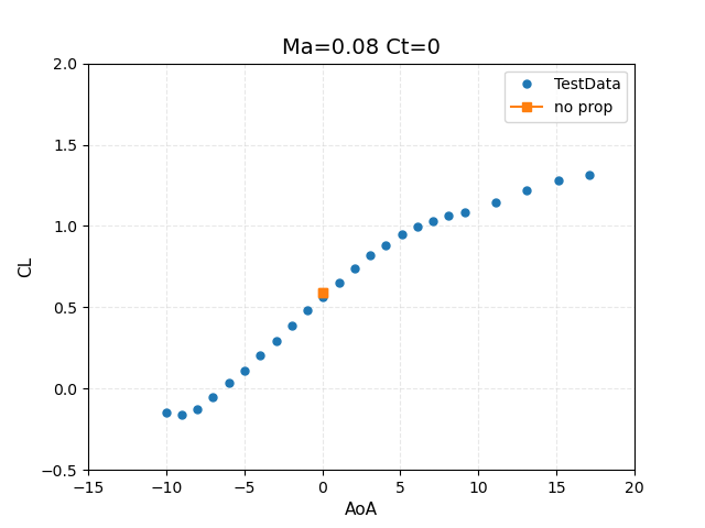
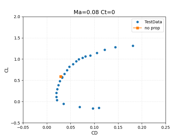
Figure 5: Comparison of power-off (CT=0.0) results with experimental data from WIPP wind tunnel test.
Next, the computed values for the powered cases are discussed. Recalling that the this case corresponds to a nominal thrust setting of CT=0.4, we have the following results:
- Assumed (linear) loading case (Case 1):
- Thrust = 18.17 lb
- Torque = -4.158 ft*lb
- CT = 0.40
- CL = 0.6764
- CD = 0.0327
- CDWA = -CT + CD = -0.3673
- Prescribed loading case (Case 2):
- Thrust = 20.4 lb
- Torque = -4.70 ft*lb
- CT = 0.448
- CL = 0.6852
- CD = 0.0340
- CDWA = -CT + CD = -0.4140
- Blade-element loading case (Case 3):
- Thrust = 19.27 lb
- Torque = -4.68 ft*lb
- CT = 0.424
- CL = 0.6988
- CD = 0.0313
- CDWA = -CT + CD = -0.3927
- Collective = 28.43 deg
- Blade-element loading case trimmed to CT=0.400 (Case 4):
- Thrust = 18.17 lb
- Torque = -4.206 ft*lb
- CT = 0.400
- CL = 0.6919
- CD = 0.0315
- CDWA = -CT + CD = -0.3685
- Initial Collective = 28.43 deg
- Final Collective = 27.12 deg
These results are plotted against the experimental data in terms of lift and drag coefficients in Figure 6, and the CDWA coefficient, which includes the (predicted) thrust component, in Figure 7.
For the assumed load distribution (Case 1), the thrust is specified in the input file as T = 18.17 lbs, which corresponds to the nominal thrust setting of CT = 0.400
For the prescribed loading case (Case 2), the computed dimensional thrust and torque values are within 1% of the values reported experimentally given by integrating the loads obtained by the wake survey (experimental values: T = 20.2 lbs, Q = 4.74 ft*lbs). This is to be expected, as the actuator disk is simply integrating the experimentally prescribed loads in this case. Nevertheless, the agreement provides verification that the loads are correct and the distribution of sources in the CFD mesh produce an accurate integration. The thrust coefficient CT is computed using the given dynamic pressure of 9.68 psf, and the reference area of 675.6 in^2. Note that the resulting value is higher than the nominal value of CT = 0.4. However, this is not a predicted value, but rather a direct result of the experimentally given loads and reference values. This discrepancy was noted in the workshop summary. The CL and CD values compare well with experiental data as shown in Figure 6. However, the value of CDWA in Figure 7 is affected by the higher CT value as discussed above.
Results for the blade element loading (Case 3) show slightly lower thrust and torque levels, with a resulting thrust coefficient that is closer to the nominal value of CT = 0.4. The predicted torque value (Q = 4.68 ft*lbs) is also close to the experimental value. In this case, these values are predicted rather than prescribed. The force coefficients are in reasonable agreement with the experimental data, and the CDWA value is closer as well, largely due to the lower predicted value of CT.
Finally, Case 4 adds trim control to the settings of Case 3, where the thrust level is specified at T = 18.17 lbs, corresponding to CT = 0.400. The collective blade pitch angle is automatically adjusted during the run to match the prescribed thrust level, and is reduced from 28.43 degrees to 27.12 degrees. The predicted torque value also decreases from Q = 4.68 ft*lbs in Case 3 to Q = 4.206 ft*lbs, as may be expected for a rotor with lower thrust and blade pitch angle. Overall, the CDWA results are closer to experimental values largely due to the correct thrust level. However, the blade collective pitch angle now differs slightly from the actual blade pitch use in the experiement.
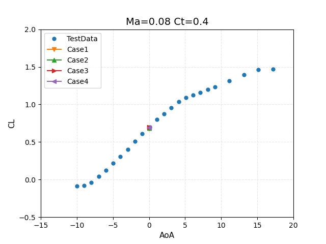
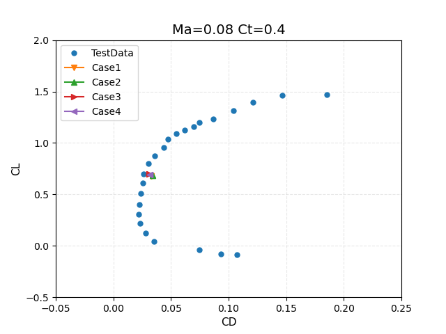
Figure 6: Comparison of computed lift and drag coefficients for CT=0.4 thrust setting with experimental data from WIPP wind tunnel test.
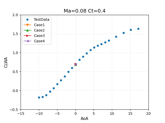
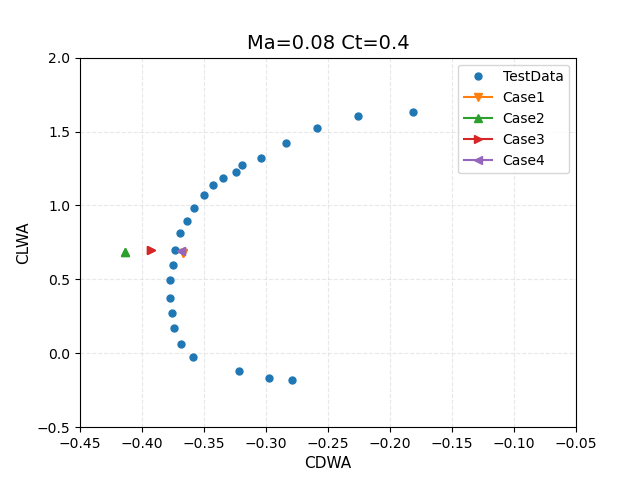
Figure 7: Comparison of force coefficients for CT=0.4 thrust setting including computed thrust with experimental data from WIPP wind tunnel test. (Note CL=CLWA in this case since there is no thrust component in the vertical direction at 0 angle of attack)
The results as plotted in AIAA paper 2022-1678 are reproduced below, where the full drag polar has been computed. Here is should be noted that only the single-point results in Figure 7 from Case 2 and Case3 correspond to curves NSU3D AD NP0.7 and NSU3D BE NP0.7, respectively.
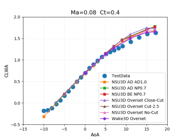
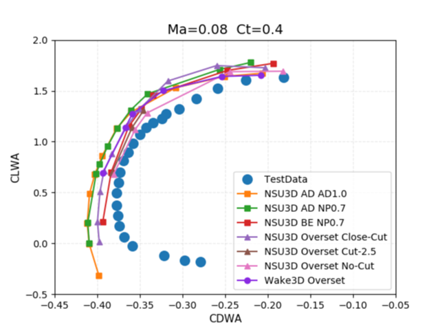
Figure 8: Comparison of force coefficients computed in AIAA Paper 2022-1678 for CT=0.4 thrust setting with experimental data from WIPP wind tunnel test.
Other Considerations
It should be noted that the above results were run at standard sea-level conditions. The workshop included the specification of a reference dynamic pressure of 9.68 psf to be used in the CFD calculations. However, for standard sea-level conditions, with a freestream Mach number of 0.08, the corresponding dynamic pressure is found to be 9.45 psf (about 2.5% lower). Although this is a relatively small difference, it impacts the value of CT which is considerably larger than the CD value, producing appreciable changes in CDWA.
Alternatively, the freestream conditions for the experimental test case can also be found in the literature for the workshop data. However, here again differences between computed and specified dynamic pressure reference values are noted. As a numerical experiment, the same cases were rerun with the experimental freestream values and using the resulting dynamic pressure for scaling. This also provides an example case of how to specify dimensional freestream or reference values.
Before showing these results, we discuss the expected changes in the results of both loading methods. For the prescribed loading case, the computed dimensional thrust should remain the same regardless of freestream values, since this is a result of the prescribed dimensional loads. However, the thrust coefficient will change due to changes in the reference dynamic pressure with different freestream dimensional values. Since the flow solver operates in non-dimensional quantities, this result in slightly different flowfield values (i.e. wake and CL CD).
On the other hand, for the blade-element method, changes in the freestream dimensional density will not affect the flowfield, since all flowfield calculations, including the blade-element calculations, are non-dimensional. However, the reported dimensional thrust and torque values will be different, while the thrust coefficient will remain unchanged. Conversely, changes to the dimensional reference velocity will affect both the flow field and the thrust and torque values and coefficients. This is due to the fact that the reference velocity is also used to scale the blade rotation rate in the blade-element method (i.e. corresponding to a fixed blade tip Mach number), thus changing the local relative velocity of the blade in this case.
For RUN180 in the workshop, the following freestream values are given:
- Freestream Density* = 0.0023 slug/ft^3
- Freestream Velocity* = 92.77 ft/sec
- Area = 675.6 in^2 = 4.692 ft^2
Note this corresponds to a freestream dynamic pressure of 9.897 psf, although the lower value of 9.68 psf was used throughout for the CFD runs in the workshop.
These values can be specified in the input.actdisk file by adding them in the actdisk_info namelist section as:
1  !WIPP BLADE-ELEMENT CASE
2  ! Initialization namelist using specific test reference values
3  &actdisk_info
4    nsystem            = 1,
5    nrotor             = 1,
6    nblade             = 1,
7    nairfoil           = 7,
8    ref_density        = 1.18537
9    ref_velocity       = 298.677
12   ref_length         = 1.0,  ! L_physical / L_grid
13   ref_length_unit    = "in"
14   show_rotor         = .true.,
15   force_output_unit  = "lb",
16   moment_output_unit = "lb*ft"
19 /
Here, SI units are assumed for the reference values as defaults. Alternatively, these values can be specified directly in imperial units as:
1  !WIPP BLADE-ELEMENT CASE
2  ! Initialization namelist using specific test reference values
3  &actdisk_info
4    nsystem            = 1,
5    nrotor             = 1,
6    nblade             = 1,
7    nairfoil           = 7,
8    ref_density        = 0.0023
8    ref_density_unit   = "sl/ft^3"
9    ref_velocity       = 980.06
9    ref_velocity_unit  = "ft/s"
12   ref_length         = 1.0,  ! L_physical / L_grid
13   ref_length_unit    = "in"
14   show_rotor         = .true.,
15   force_output_unit  = "lb",
16   moment_output_unit = "lb*ft"
19 /

..
Note that the reference velocity corresponds to the (freestream speed of sound)/sqrt(gamma). Therefore, the freestream velocity given experimentally is divided by the Mach number to obtain the freestream speed of sound, and then the dimensional reference velocity can be obtained as above.
Given these inputs, the computed results for both cases become:
- Prescribed loading case (Case 2):
- Thrust =
- Torque =
- CT =
- CL =
- CD =
- CDWA = -CT + CD =
- Blade-element loading case (Case 3):
- Thrust =
- Torque =
- CT =
- CL =
- CD =
- CDWA = -CT + CD =