Tutorial Overview
Once the NSU3D suite is obtained and built (see Getting Started), download the tutorial files here. If your system tar command does not support inline gzip compression, then you will need to run gzip -d on each archive and then use tar xvf to unpack it.
The f6wbnc case is a standard steady-state RANS NSU3D test case.
This case consists of a sample grid files, input files, and output files.
The directories associated with this case are:
- grids
- RUN.tecform1
- RUN.pre_nsu3d
- RUN.nsu3d.FAS
- RUN.regression_test
The general procedure for setting up and running these types of cases is the following:
- Check consistency of bcs and comp files by running tecform as given in the RUN.tecform1 directory.
- Run pre_nsu3d preprocessor to preprocess and partition mesh file as shown in RUN.pre_nsu3d
- Run nsu3d as shown in RUN.nsu3d.FAS
- Postprocess using post_nsu3d and tecform as shown in RUN.nsu3d.FAS
- Run the regression test checks as shown in RUN_regression_test
The directory "grids" contains the following files:
- f6wbnc.bcs
- f6wbnc.comp
- f6wbnc.mcell
f6wbnc.bcs: Boundary condition file; associates a bctype with each patch in the mesh geometry.
f6wbnc.comp: Component file; defines components based on patches in the mesh geometry.
Integrated force coefficients are output based on components as well as bctypes.
f6wbnc.mcell: Initial (unprocessed) grid file in mixed element format (see mcell file definition in documentation).
This is an unformatted fortran file in real*8 precision.
The mcell file is the product of a grid generation procedure and is output by the grid generation software.
Various grid generation codes support the mcell format (ICEM and Pointwise NSU3D formats).
Converters are provided to convert other grid generation formats to mcell format.
pre_nsu3d also supports other file formats (vgrid and b8.ugrid:
see Compatible Model Grids for more information).
The bcs and comp files may or may not be output by the grid generation software.
In general, the bcs files output by ICEM and Pointwise work,
but may have bugs or may be formatted in an non optimal way.
Thus it is often useful to construct these by hand.
Consistency Check for bcs and comp files
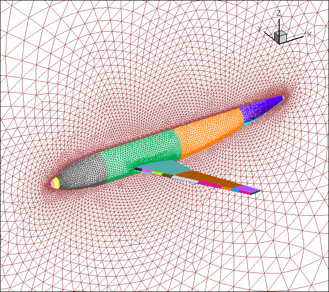
In order to pick patch numbers, and to ensure that the bcs and comp files are constructed correctly, the tecform facility can be used to check these input files prior to preprocessing the mesh. An example of this workflow is provided in the RUN.tecform1 directory. Running tecform with the provided input files as:
- tecform < input.patch.tec
produces a tecplot file which can then be viewed in tecplot where
each surface patch is identified as an individual zone in tecplot.
Similarly:
- tecform < input.bcs.tec
- tecform < input.comp.tec
produces a tecplot file where each boundary condition or each component
is identified as an individual zone in tecplot.
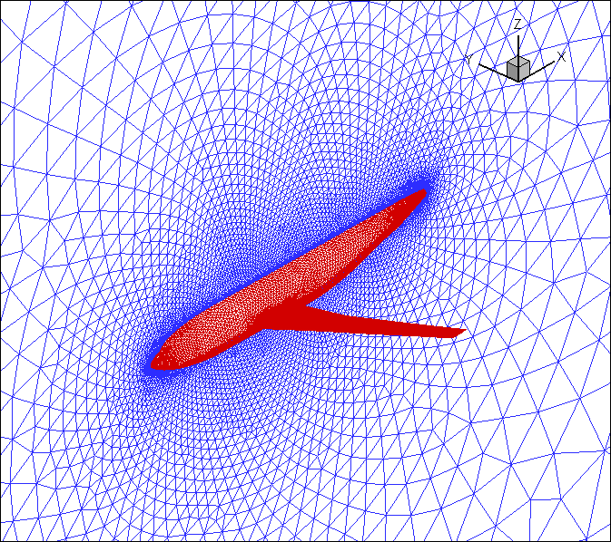
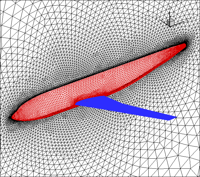
The results produced by these 3 runs are given in the subdirectory RESULTS,
including the resulting tecplot file, and a png figure (shown above) produced
using the accompanying tecplot layout file.
It is strongly recommended to run these visual checks on the bcs and comp files
prior to preprocessing the mesh and running the flow solver.
Preprocessing
An example for preprocessiing and partitioning of the mesh
is given in the directory RUN.pre_nsu3d
This is done using the pre_nsu3d code.
This can be invoked in several ways:
- Running pre_nsu3d and amg3d by hand
- Invoking the pre_nsu3d.sh script
- Using the pre_nsu3d.py script
For simplicity this example uses option 1, which also provides the user with a better understanding
of how the software works (compared to using the scripts).
In order to preprocess the f6wbnc.mcell mesh, the pre_nsu3d code is invoked
using the supplied input file: input.pre_nsu3d
This input file lists the mesh file (f6wbnc.mcell) and corresponding bcs and comp files.
The preprocessing partitions the mesh but also constructs the line data-structures
and coarse multigrid levels for the NSU3D solver and outputs all required information
in a directory with individual partition files called f6wbnc.part.n
where n is the specified number of partitions (128 in this example)
For multigrid runs, the preprocessor must be run twice when the mesh is partitioned for the first time.
On the first pass, pre_nsu3d is run to get an amg file, then amg3d is run, and then pre_nsu3d is run again:
- mpirun -np 128 pre_nsu3d input.pre_nsu3d | tee out.pre_nsu3d.1
- amg3d | tee out.amg
- mpirun -np 128 pre_nsu3d input.pre_nsu3d | tee out.pre_nsu3d.2
This creates the directory with all part files called casename.part.128
The mesh can now be repartitioned into other numbers of partitions with a single run of pre_nsu3d:
- mpirun -np 16 pre_nsu3d input.pre_nsu3d | tee out.pre_nsu3d.16part
This creates the directory with all part files called casename.part.16
Note that the mesh can be preprocessd onto a single partition using:
- mpirun -np 1 pre_nsu3d input.pre_nsu3d | tee out.pre_nsu3d.1part
This creates the directory with all part files called casename.part.1
This can be useful for debugging or comparing parallel cases with sequential runs.
Note there are 2 scripts that can run pre_nsu3d and amg3d with a single command.
However, these use a particular command for mpirun which may differ on different
computer architectures. In order to work on your specific architecture,
the command may need to be edited (in the .sh script) or set by an ENV variable
in the python script, see running pre_nsu3d for more information.
Running the Flow Solver
Now that the mesh has been preprocessed and partitioned, the flow solver can be run. From within the RUN.nsu3d.FAS directory, and using the supplied input.nsu3d file, run nsu3d as:
- mpirun -np 128 nsu3d input.nsu3d | tee out.nsu3d
This command pipes standard out to the file out.nsu3d as well as scrolling it on the screen in an interactive session. Alternatively one can run as:
- mpirun -np 128 nsu3d input.nsu3d > out.nsu3d
For this case nsu3d will run the prescribed number of iterations and place all output in the local directory called ./WRK
Postprocessing
Run the post processor in the RUN.nsu3d.FAS directory. Post processing is done in two steps:
A: Create a single image file from the partitioned restart file written out by NSU3D as:
- post_nsu3d < WRK/input.postnsu3d > out.post
Note the file input.post_nsu3d is created by NSU3D in the resulting ./WRK directory.
B: Run TECFORM to create a tecplot file for visualizing the computed surface values:
- tecform < input.tec > out.tec
C: Visualize tecplot file created above,
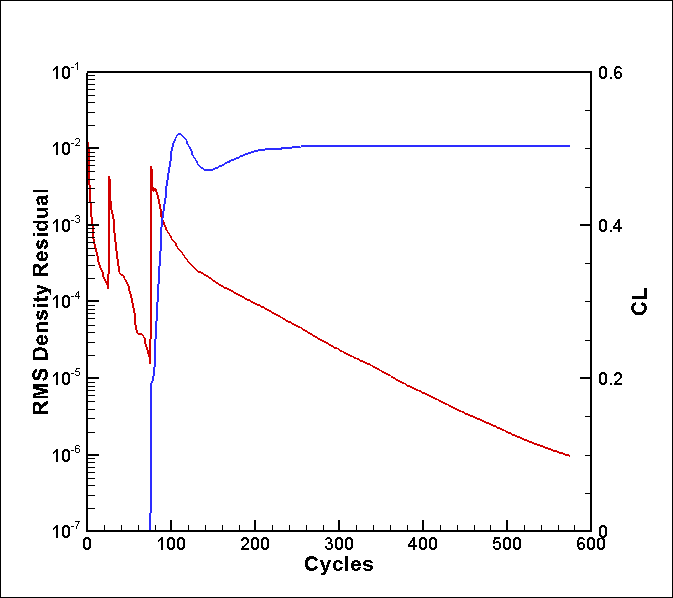
and plot convergence histories by reading the log files in ./WRK directly into tecplot.
Most common file for FAS (nonlinear) multigrid or FSOLVER=0 is: rplot.out or rplot.restart.out
For linear solvers (FSOLVER=1,2,3) use nonlinear_rplot.out/nonlinear_restart.plot.out
and linear_rplot.out/linear_rplot.restart.out
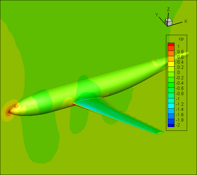
In the directory /F6.STEADY.regtest/RUN.tecform1 there are some example tecplot input files.
In the subdirectory "RESULTS", the resulting tecplot files and produced png figures (shown below)
using the corresponding tecplot layout files are provided for comparison.
Regression Test
A regression test is provided to verify that the users given architecture and compiled code gives
the correct solution. This regression test uses the results of the above F6wbnc Steady tutorial test
case and requires the user to follow the instructions exactly, specifically with naming output files and folder locations.
In the RUN.regression_test folder is a script to run tests on nsu3d: pre-processor, flow solver, post-processor. The tests compare
output file statistics, grid header files, solution surface forces, and tecform ascii files.
After completing the tutorial above the regression test is run using
- ./nsu3d_regression_test.bash